Mock Project


Hello guys. So, as part of my MS Excel learning journey, I had to complete a mock project. I’ll be sharing some screenshots of the project here.
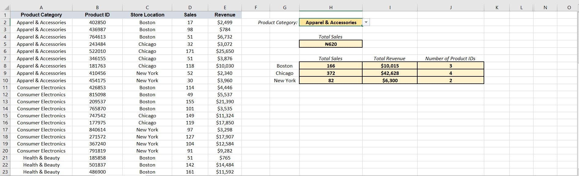
Here, I had to populate the cells formatted in yellow. For the product category cell, I created a dropdown list containing the items in column A using Data Validation. For the total sales cell, the result is based on what is in the product category cell. So, I used the SUMIF function with cell H2 (product category) as the criterion.
For the remaining cells, I used the SUMIFS function, with the product category cell and the cells listing Boston, Chicago, and New York as the criteria.
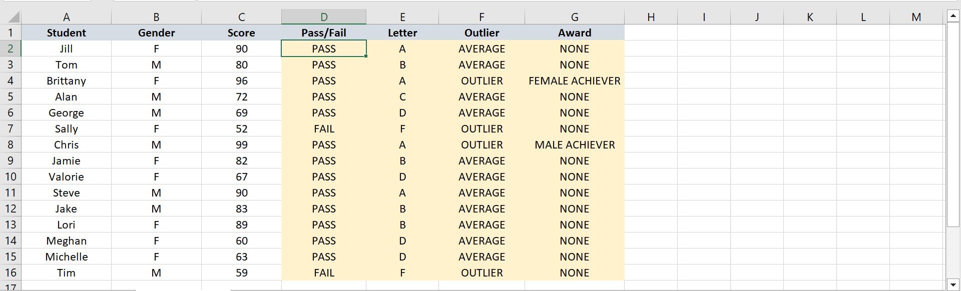
Here, I used the IF function to populate column D, with 60 and above for PASS, and below 60 as FAIL. For column E, I used NESTED IFS to populate it, with A\>=90, B = 80-89, C = 70-79, D = 60-69, and F = <60.
I used the IFOR function to populate column F test scores less than 60 or greater than 90 returning “OUTLIER”, and any score in between returning “AVERAGE”.
For column G, I used the IFAND function. A score above 95 and gender “M” returns “MALE ACHIEVER”. If it’s gender “F”, it returns “FEMALE ACHIEVER”.
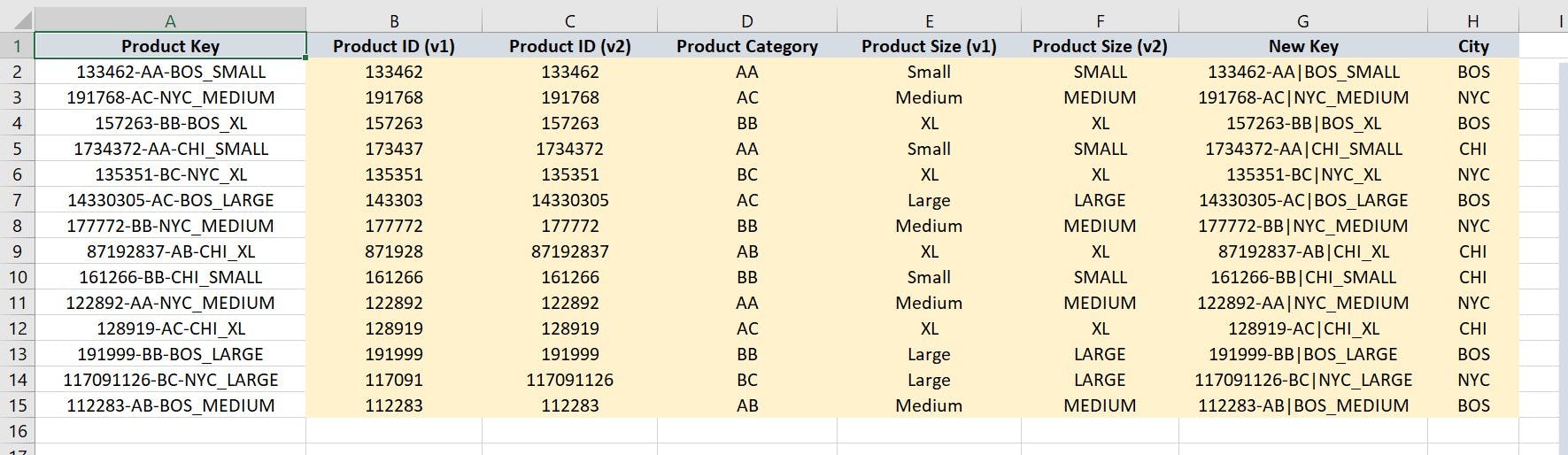
For this, I populated the formatted cells with the data in column A. I’ll talk about just columns E and F. I used different combinations of functions to achieve the same result. The product size is at the end of the product key in column A.
For column E, I used a combination of the IF, ISNUMBER, and SEARCH functions. Here’s the formula:
=IF(ISNUMBER(SEARCH("small",$A2)),"Small",IF(ISNUMBER(SEARCH("medium",$A2)),"Medium",IF(ISNUMBER(SEARCH("large",$A2)),"Large",IF(ISNUMBER(SEARCH("xl",$A2)),"XL"))))
For column F, I used a combination of the RIGHT, LEN, and SEARCH functions. Here’s the formula:
=RIGHT($A2,(LEN($A2)-SEARCH("_",$A2,1)))
I’ll stop here. But really, I must say, it was exciting to work on this. I relished that feeling of writing out a formula, actually understanding it, and watching it work.
See ya.